An approximation algorithm returns a solution to a combinatorial optimization problem that is provably close to optimal (as opposed to a heuristic that may or may not find a good solution). Approximation algorithms are typically used when finding an optimal solution is intractable, but can also be used in some situations where a near-optimal solution can be found quickly and an exact solution is not needed.

Many problems that are NP-hard are also non-approximable assuming P≠NP. There is an elaborate theory that analyzes hardness of approximation based on reductions from core non-approximable problems that is similar to the theory of NP-completeness based on reductions from NP-complete problems; we will not discuss this theory in class but a sketch of some of the main results can be found in (Vijay V. Vazirani, Approximation Algorithms, Springer, 2001), which is also a good general reference for approximation. Instead, we will concentrate on some simple examples of algorithms for which good approximations are known, to give a feel for what approximation algorithms look like.

The quality of an approximation

In any combinatorial optimization problem, there is some objective function we are supposed to optimize. The approximation ratio (or approximation factor) of an algorithm is the ratio between the result obtained by the algorithm and the optimal cost or profit. Typically this ratio is taken in whichever direction makes it bigger than one; for example, an algorithm that solves for a cost of $2 an instance of a problem that has an optimal cost of $1 has approximation ratio 2; but an algorithm that sells 10 airplane tickets (a profit of 10) when the optimum is 20 also has approximation ratio 2.

An algorithm with approximation ratio k is called a k-approximation algorithm; both algorithms above would be called 2-approximation algorithms.

When the approximation ratio is close to 1, it is often more useful to look at the approximation error, which is defined as the approximation ratio minus 1. So an algorithm that always got within 1.01 of the optimal cost or profit would have a 1% approximation error.

A family of algorithms that can achieve any constant approximation error in polynomial time is called a polynomial-time approximation scheme or PTAS. A family of algorithms that can achieve any approximation error ε>0 in time polynomial in both 1/ε and n is called a fully polynomial time approximation scheme or FPTAS. Fully polynomial-time approximation schemes are the holy grail of approximation algorithms; they do not appear to exist for many problems, but when they are available, they are often almost as useful as an optimizing algorithm would be.

Proving an approximation ratio

In general, proving that an algorithm gives a good approximation ratio is hard. It's not enough to prove that the algorithm's output is good (which we usually know how to do); you also have to show that the optimum is not much better. This takes us into the realm of proving lower bounds, which can be tricky when we can't figure out what the optimum should be. Most of the time a crude lower bound can be obtained from the structure of the problem (see the VERTEX COVER approximation below); occasionally the solution method also helps (for example, a fractional solution to a linear program gives a lower bound on the quality of the best integer solution).

Vertex cover

The minimum vertex cover problem on a graph asks for as small a set of vertices as possible that between them contain at least one endpoint of every edge in the graph. It is known that vertex cover is NP-hard, so we can't really hope to find a polynomial-time algorithm for solving the problem exactly. Instead, here is a simple 2-approximation algorithm:

ApproximateVertexCover:
  while there are unmarked edge
    choose an unmarked edge
    mark both its endpoints

To show that this gives a 2-approximation, consider the set E' of all edges the algorithm chooses. None of these edges share a vertex, so any vertex cover must include at least |E'| vertices. The algorithm marks 2|E'| vertices.

Traveling Salesman

The input to the traveling salesman problem (TSP) is an undirected graph with edge weights, and the optimal output is a cycle that visits every vertex exactly once (a tour) with minimum total weight. It is not possible to find such a tour in polynomial time unless P=NP, because there is an easy reduction to the decision version of TSP (does G have a tour of length k or less?) from the NP-complete problem HAMILTONIAN CIRCUIT, which asks if any tour exists of any weight. Set weight 1 for all edges in the original HAMILTONIAN CIRCUIT GRAPH, and weight M for all other pairs of vertices, and let k = |V|. Since the any invalid tour in this graph has total weight at least M-|V|+1, and M can be made arbitrarily large, we have in fact showed that there is in general no polynomial-time r-approximation to TSP for any fixed r unless P=NP.

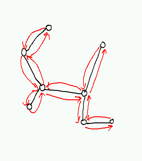
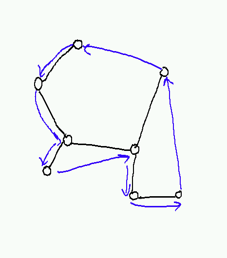
However, for edge distances that satisfy the triangle inequality d(x,y) ≤ d(x,z) + d(z,y) for all x, y, z, there is a 2-approximation algorithm based on MinimumSpanningTree. Construct an MST T of the graph G, and generate a cycle C that traverses T in depth-first order.

This cycle is not a tour, because it visits non-leaf nodes more than once. We can make it a tour by deleting the second occurrence of any non-leaf node (except the root), and replacing the edge or edges used to traverse these missing nodes by a single edge between the previous and next nodes that are not removed. This gives us a tour C'; by the triangle inequality, the new edges are no longer than the paths they replace, so length(C') ≤ length(C).

But how long is C? We have length(C) = 2 length(T). Consider any optimal tour C^*. Remove any edge from C^* and we have a (very linear) spanning tree. It follows that length(T) ≤ length(C^*) and thus that length(C') ≤ 2 length(T) ≤ 2 length(C^*), giving an approximation ratio of 2 as claimed.

For Euclidean TSP, where the vertices are embedded in some Euclidean space (e.g. the plane) and the edge weights are the usual Euclidean distances, there is a FPTAS due to Arora (see http://citeseer.ist.psu.edu/arora96polynomial.html).

Knapsack

Recall that the KnapsackProblem is to find, given a set of items S with given weights w_i and profits p_i and a bound k, a subset S' that maximizes ∑_{i in S'} p_i subject to the constraint ∑_{i in S'} w_i ≤ k. Though knapsack is NP-complete, there is a fully polynomial-time approximation scheme for knapsack based on rounding.

The basic idea is that we can solve knapsack in O(nP) time by DynamicProgramming if (a) all profits p_i are integers and (b) ∑_{i in S} p_i ≤ P. Number the elements of S from 1 through n and let w(p,k) be the minimum weight of any subset of items 1 through k with total price p. To get a total price p from 1..k, we either take item k or not; the minimum weight is given by

• w(p,k) = min(w(p,k-1), w(p-p_k,k-1) + w_k).

with the base case

• w(0,0) = 0; w(p,0) = ∞ for p > 0.

We can easily compute a table of all w(p,k) values in O(nP) time using dynamic programming; we then take the maximum p for which w(p,n) ≤ k and reconstruct the corresponding S'.

What do we do if ∑_{i in S} p_i is large? We can rescale all of the weights by defining

• p'_i = p_i(P/∑p_i)

which yields ∑p'_i = P. This gets (b), but it doesn't get (a); the weights p'_i are not integers. So we further define

• q_i = ⌊p'_i⌋ = ⌊p_i(P/∑p_i)⌋

and then solve knapsack for the original weights w_i and the truncated scaled weights q_i.

The resulting solution maximizes ∑_{i in S'} q_i; no other solution improves on this quantity. But the q_i do not contain all the information about the profits, and it is possible that some other S^* has higher ∑_{i in S*} p'_i. But this sum can't be too much higher than ∑_{i in S'} p'_i; to see this, observe than

• p'_i < q_i + 1 for all i,

so

• ∑_{i in S*} p'_i < n + ∑_{i in S*} q_i ≤ n + ∑_{i in S'} q_i.

It follows that the total profit of the optimal solution (after scaling) is less than n units greater than the total profit of the solution found by the approximation algorithm.

To show a low approximation error, we have to show that this difference total profit is small relative to the total profit of the optimum. The worst case is when the optimum is small (because this makes the ratio big). But we can (very crudely) bound the optimum by observing that the worst we can do is to take the most expensive object, whose value is at least the average value:

• ∑_{i in S*} p'_i ≥ max_{i in S} p'_i ≥ (1/n) ∑_{i in S} p'_i = P/n.

So we have:

• (difference in profit)/(optimal profit) ≤ n/(P/n) = n²/P.

If we solve for P given a particular ε = n²/P, we get P = n²/ε, so O(nP) = O(n³/ε), which is polynomial in both n and 1/ε as required.

Rounding techniques like the above can often be used to find approximation schemes for many problems that have good "fixed-parameter" solutions, where (as in this case) the solution is not hard as long as some of the parameters are kept small. Rounding also plays a role in problems that can be expressed as integer linear programs (see LinearProgramming); in this case, a fractional solution to the linear program is rounded to a nearby integer solution, and the approximation ratio can often be obtained by using the quality of the fractional solution as a lower bound on the quality of the optimal integer solution. For more on these techniques see the Vazirani book mentioned previously.

---

CategoryAlgorithmNotes