Basics of depth-first search. We'll be describing it in recursive form. To see what it would look like in iterative form with an explicit stack, see BreadthFirstSearch or C/Graphs.

1. Depth-first search in a tree

Let's start with a tree:

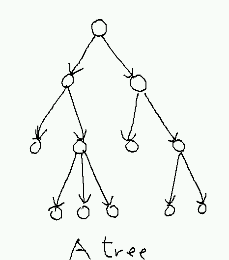
A depth-first search traversal of the tree starts at the root, plunges down the leftmost path, and backtracks only when it gets stuck, returning to the root at the end:

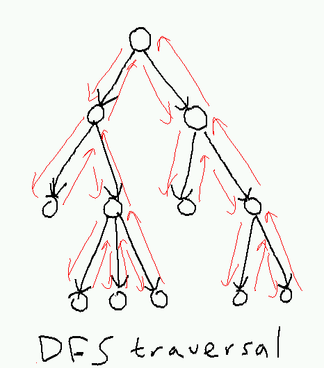
Here's a recursive implementation:

TreeDFS(root):
  // do anything we need to do when first visiting the root
  for each child of root:
    TreeDFS(child)
  // do anything we need to do when last visiting the root

The running time of TreeDFS on a tree with n nodes is given by

• T(n) = Θ(1) + ∑_i T(k_i)

where k_i is the size of the subtree rooted at the i-th child of the root. This is one of these recurrences that isn't fully defined, since we don't know in general what the values of the k_i are. But we do know that the sum of the k_i must be n-1 (the one is the root node). So if we guess that T(n') ≤ cn' for n' < n, we can compute

• T(n) ≤ an + ∑_i T(k_i) ≤ an + ∑_i ck_i = an + c ∑_i k_i = an + c(n-1) ≤ cn,

provided a ≤ c.

What can we do with TreeDFS? If we pass along some additional information, we can compute backpointers:

TreeMakeBackPointers(root, parent):
  parent[root] = parent
  for each child of root:
    TreeMakeBackPointers(child, root)

Or we can compute start and end times for each node. Here clock is a global variable initialized to zero.

TreeTimes(root):
  start[root] = clock; clock = clock + 1
  for each child of root:
    TreeTimes(child)
  end[root] = clock; clock = clock + 1

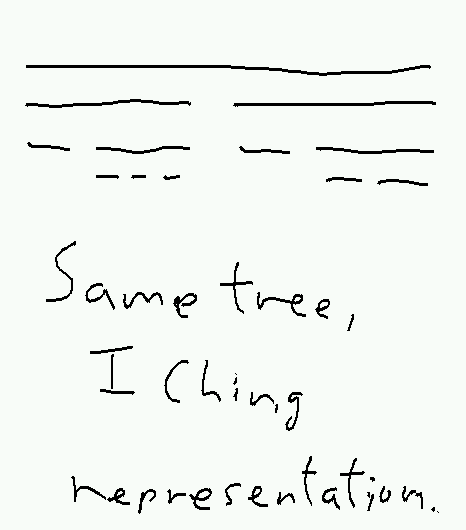
These times can be used to quickly test if one node is a descendant of another. The rule is that if x is a descendant of y, then start[y] < start[x] < end[x] < end[y]. This gives another picture of the tree, where each node is drawn as an interval:

2. Depth-first search in a directed graph

What happens if we have a graph instead of a tree? We can use the same algorithm, as long as we are careful never to visit the same node twice. This gives us the standard depth-first search algorithm. We assume that we have an array visited whose entries are initialized to false.

DFS(u):
  visited[u] = true
  for each successor v of u:
    if not visited[v]:
       DFS(v)

Here a successor of a node u is any node v for which uv appears in the set of edges of G.

An immediate application of DFS is testing reachability. If we call DFS starting with some node s, the set of nodes that are marked as visited will be precisely those nodes u for which a directed path from s to u exists in G. Note that this will give different results depending on which node s we start with.

With the graph version of DFS, only some edges (the ones for which visited[v] is false) will be traversed. These edges will form a tree, called the depth-first-search tree of G starting at the given root, and the edges in this tree are called tree edges. The other edges of G can be divided into three categories:

• Back edges point from a node to one of its ancestors in the DFS tree.

• Forward edges point from a node to one of its descendants.

• Cross edges point from a node to a previously visited node that is neither an ancestor nor a descendant.

This classification of the non-tree edges can be used to derive several useful properties of the graph; for example, we will show in a moment that a graph is acyclic if and only if it has no back edges. But first: how do we tell whether an edge is a tree edge, a back edge, a forward edge, or a cross edge? We can do this using the clock mechanism we used before to convert a tree into a collection of intervals. If we also compute parent pointers along the way, we get a version of DFS that is usually called annotated DFS:

AnnotatedDFS(u, parent):
  parent[u] = parent
  start[u] = clock; clock = clock + 1
  visited[u] = true
  for each successor v of u:
    if not visited[v]:
      AnnotatedDFS(v, u)
  end[u] = clock; clock = clock + 1

Tree edges are now easy to recognize; uv is a tree edge if parent[v] = u. For the other types of edges, we can use the (start,end) intervals to tell whether v is an ancestor, descendant, or distant cousin of u:

For tree, back, and forward edges, the relation between the start times and end times of the endpoints is immediate from the tree structure. For cross edges, knowing only that u is neither and ancestor nor descendant of v tells us only that u and v's intervals do not overlap. But we can exclude the case where u's interval precedes v's interval by observing that if u's end time precedes v's start time, then v is not marked as visited when AnnotatedDFS considers the edge uv; in this case v will become a child of u, and uv will be a tree edge and not a cross edge.

Note that every edge goes backward in end time except for back edges. If we have no back edges, then if we sort the nodes by reversed end time, all edges go from an earlier node in the sorted list to a later node. This almost gives us an algorithm for TopologicalSort; the complication is that AnnotatedDFS above may not reach all nodes.

3. DFS forests

The solution is to attach a "virtual root" to the graph from which all nodes are reachable. This guarantees that DFS visits and assigns parent pointers and start and end times to all nodes. The result of running DFS (if we ignore the virtual root) is now a DFS forest---a collection of one or more DFS trees that may be linked by cross edges.

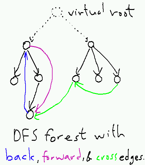
In practice, we do not represent the virtual root explicitly; instead, we simply replace the loop over all of its successors with a loop over all vertices. So instead of starting the search with a call to AnnotatedDFS(root, nil), we use a specialized top-level function AnnotatedDFSForest:

AnnotatedDFSForest:
  for u = 1 to |V|:
    if not visited[u]:
      AnnotatedDFS(u, nil)

Given an undirected graph, we will have no cross edges (they will become tree edges in the other direction instead), and the DFS forest will consist of exactly one tree for each connected component of the original graph. Thus DFS can be used to compute ConnectedComponents, for example by marking the nodes in each tree with a different mark.

The same arguments about edge types and direction with respect to start and end times apply in the DFS forest as in a single DFS tree. So we can solve TopologicalSort for the entire graph by simply running AnnotatedDFSForest and then sorting by reversed end times. If we are not promised that the input is acyclic, we can test for this as well by looking for back edges.

4. Running time

Checking whether the endpoints of all of the non-tree edges have been visited already may raise the cost of DFS above the Θ(n) cost of the tree-only version. But we can write a slightly modified version of the recurrence for TreeDFS by taking advantage of the DFS tree. Let T(V,E) be the running time of DFS on a node whose subtree contains V vertices that between them have E outgoing edges. Then

• T(V,E) = Θ(1) + Θ(d) + ∑_i T(V_i, E_i)

where d is the degree of the root (the number of edges leaving the root), and for each child i of the root in the DFS tree, V_i and E_i are the number of vertices and outgoing edges in the subtree rooted at that child. As before, we have ∑_i V_i = V - 1; we also have ∑_i E_i = E - d. If we conjecture that T(V,E) = O(V+E), we can prove it by computing

• T(V,E) ≤ a + ad + ∑_i T(V_i, E_i) ≤ a + ad + ∑_i c(V_i+E_i) = a + ad + c ∑_i V_i + c ∑_i E_i = a + ad + c(V-1) + c(E-d) ≤ c(V+E),

again provided a ≤ c.

This analysis shows that the simple AnnotatedDFS runs in time Θ(V+E) where V and E are the number of vertices and edges reachable from the starting node. For AnnotatedDFSForest, we can apply the same analysis to the graph with the added virtual root, giving Θ(V+E) time where V and E are now the number of vertices and edges in the entire graph. It follows that depth-first search is a linear time algorithm, where the time is computed as a function of the size of the input.

5. A more complicated application: strongly-connected components

A strongly-connected component of a directed graph G is a maximal subset V' of the vertices with the property that every node in V' is reachable from every other node in V'. What makes strongly-connected components different from connected components in undirected graphs is that in an undirected graph, if you can reach v from u, you can go backwards along the same path to reach u from v; but in a directed graph, it may be that you can reach v from u but not be able to go back. An extreme case is an acyclic graph. In an acyclic graph, you can never go home again, and every node by itself is a strongly-connected component, even though there may be many edges between nodes.

Finding the strongly-connected components is thus closely related to finding cycles. We have already seen that we can detect cycles by looking for back edges in a DFS forest. So to find strongly-connected components, we will first compute a DFS forest and then look for chains of back edges that take us up higher in the tree. Each strongly-connected component we find will be identified with some highest reachable node, and will consist of all descendants of that node that can reach it by some path.

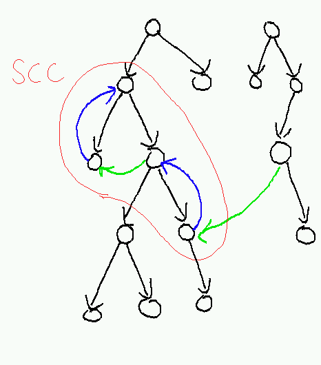
Let's formalize this notion of the highest reachable node. We will use the end times computed during the execution of AnnotatedDFSForest. Let H(u) be the node with the highest end time among all nodes reachable from u (including u itself).

Lemma

H(u) is an ancestor of u.

Proof

Surprisingly painful. The intuitive (i.e. not rigorous enough to actually be convincing; for a real proof that this algorithm works, see CormenEtAl) argument goes like this: Consider all pairs (u,H(u)) where H(u) is not an ancestor of u, and choose u to minimize the length of the shortest path from u to H(u). Then if the first edge on this shortest path is uv, we have H(u) = H(v) which is an ancestor of v. It follows that uv can't be a back edge or tree edge, or else H(v) = H(u) would be an ancestor of u. It's also the case that uv can't be a forward edge, because the either H(u) would be an ancestor of u or a proper descendant of u; in the second case end[H(u)] < end(u), contradicting the assumption that H(u) maximizes the end time. So uv must be a cross edge. But then v is in an earlier part of the tree than u, and if H(v) is not an ancestor of u we must have end[H(v)] < start[u], again contradicting the assumption of maximal end time.

Corollary

H(u) = H(v) if and only if u and v are in the same strongly-connected component.

Proof

If H(u) = H(v), then u -> H(u) = H(v) -> v is a u-v path. Conversely, if u and v are in the same strongly-connected component, then any node reachable from u is reachable from v and vice versa. It follows that the node with the latest end time reachable from u is the node with the latest end time reachable from v, i.e. H(u) = H(v).

So how do we compute H(u) for each u? There is a simple algorithm that runs DepthFirstSearch twice:

StronglyConnectedComponents(G):
  Run AnnotatedDFSForest on G.
  Let G' equal G with all edges reversed and the vertices ordered by decreasing end time.
  Run AnnotatedDFSForest on G' and output each tree as a SCC.

Why this works: The first call to DFS computes the end times. When we run in the reverse direction, we are computing the set of nodes that can reach each node. A node will only appear as the root of a tree in the forest if it can't reach any node with a higher end time; i.e. if it's the high end-time node for some component.

If we only want to know if there is a single strongly-connected component, i.e. if the graph itself is strongly connected, there is a simpler algorithm:

IsStronglyConnected(G):
  Run DFS on G starting at some node s.
  If some node is not marked, return false.  (It is not reachable from s).
  Run DFS on G' starting at s, where G'is G with all edges reversed.
  If some node is not marked, return false.  (It cannot reach s).
  If we haven't returned anything yet, return true.

This also has linear-time running time in the worst case, but may be faster that the previous algorithm if the graph is not strongly connected and s can't reach very many nodes. It is easier to see why this works; if we return false, it's because we found a node t with either no s-t path or no t-s path. If we return true, then every node can reach s and s can reach every node; so between each pair of nodes u and v there is a path u->s->v (and possibly other, better paths), which is enough to show strong connectivity.

---

CategoryAlgorithmNotes CategoryProgrammingNotes